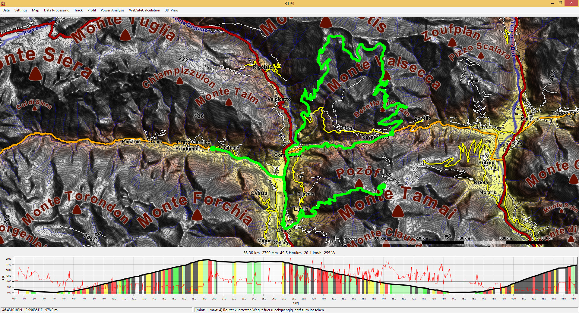
The BergTourenPlaner (BTP, English: climb tour designer) is a offline tool to plan tours, estimated power output, estimate time tables for a given route, find tours with the highest/least altitude gain, find climbs and create 3D-views. BTP is an open source project combining open source road network data of OpenStreetMap and the SRTM3 digital elevation model of the NASA. The contents of climbindex.eu were generated with BTP.
Following the advices you might be soon ready to analyse the massive stage final which had been once planned at the Giro d'Italia but than shortened to the zoncolan only due to riders striking
If the program does not start any more, try to delete the settings.stg file within the application folder.
| ↑ (up) | navigate to the north |
| ↓ (down) | navigate to the south |
| ← (left) | navigate to the west |
| → (right) | navigate to the east |
| + (plus) | zoom in |
| + (minus) | zoom out |
| ESC | delete track; if STRONG is calculating: stop calculation |
| delete | delete track; if STRONG is calculating: stop calculation |
| ↵ (enter) | start an "open end" routing. Lock a previewed track pressing 'n', accept it with a further enter press. Or just click by mouse instead. |
| ⇐ (backspace) | delete last segment of the track; press ctrl atditionally to delete last 10 segments |
| ⇑ (page up) | select among the pareto optimal STRONG tracks after a successful STRONG calculation |
| ⇓ (page down) | select among the pareto optimal STRONG tracks after a successful STRONG calculation |
| F5, F6, F7, F8 | switching active elevation date to SRTM3, SRTM1, SRTM066 or SRTM018. Before using any elevation data (Digital elevation modell, DEM) you have to specify data folder in "settings" menu. Be aware that using high-resolution data (SRTM018 means 0.18 arc seconds, i.e. a data grid with max. 5.5 Meter spacing) requires larger amount of RAM if shown area becomes too large. A common problem is working with SRTM018 one day, an the other you'de like to load a gpx file which covers a much larger area: in this case BTP may fail to load due to insufficient RAM resources to render the map below the track. |
| ^,1,2,3,4,5,6,7,8,9,0 | set maximum allowed track type, press ctrl to set minimum track type: 0 motorway, 1 national highway, 2 main road, 3 side road, 4 small road (usually still tarmaced), 5 tracks good, 6 tracks medium, 7 tracks bad, 8 paths good, 9 paths medium, 10 paths bad |
| a | travelling sales man routing; 1. save desired track which should be reached using menu "track->save btr", 2. (optional) choose start point, 3. either choose end point (if start was specified before) or hit enter, 4. select the previously saved tracks in the dialogue |
| b | route for highest Hm/km quotient, 'mountain mode', adjust algorithm in 'Settings->STRONG settings' |
| c | route for most climbing per km, 'climb mode', adjust algorithm in 'Settings->STRONG settings' |
| ctrl+c | coordinate to clipboard |
| e | editing mode, allows to select map elemens and delete or modify its type with the numbers |
| f | route for least accumulated height difference, 'flat mode' |
| g | 'go to' dialog to change map position, moves to lat/lon coordinates given in degree |
| k | route short, 'kurz mode'; pressing ctrl at mouse click leads to air-line routing, creates new points in data base to insert new track. I you'de like to snap to a arbitary point on a way you first need to create a crossroad on that way |
| l | select layer, generates STRONG layer from a finished STRONG calculation |
| m | used only marked routes for routing (hike or bike routes), you may switch to hike map view ('Map -> toggle Hike-Bike') to see trail marking |
| n | toggles preview: within any routing mode you have the possibility to press ENTER instead of choosing an end point with mouse. You then can move the mouse over the map and the specified track will be shown instantly. press 'n' to lock this view or unlock. Press Enter or click with the mouse to accept this track. |
| r | ignore/apply traffic restrictions in routing: distance/time penalties in case of traffic lights, right of way, stop signs etc. |
| s | route STRONG, calculates shortes tracks at give maximum give accumulated altitude gain, 'STRONG mode', for details see STRONG, adjust algorithm in 'Settings->STRONG settings' |
| t | route for shortest time (a longer way through a valley might be faster than the short hilly track), 'time mode', time is calculated by the current Settings of the Power Analysis Window |
| y | redo (last track modification) |
| z | undo (last track modification) |
| Data→load btp | loads new map data and adds it to the existing data. By that you might combine data sets |
| Data→save btp | saves all loaded map data, which is currently shown. Zoom and move the map (and reload the data subsequently) to cut the data to the desired region. Cutting an existing dataset is the most important thing you should consider when aiming for faster operation of BTP. |
| Data→read osm | reads a *.osm file and generates map data from it. This task may take up to an hour time. osm-files up to an 2 Gb may be read. There size of your available memory should be at least as big as the osm-file. |
| Data→close | close the BTP |
| Data→analyse gpx/fit | loads a gpx-file or a fit file. You can choose whether the elevation data should be recalculated by BTP. This gpx-Analysis might be interesting in terms of forecasting times and speeds at a given track as well as estimating the power with regard on the time stamps of the gpx. Press 'Ignore time stamp' in the Power Analysis window to use the user specified Power-velocity dependence instead of time stamps. Any gpx-file you may 'open with' BTP from the explorer, as BTP accepts command line arguments |
| Settings→SRTM3 data folder Settings→SRTM1 data folder Settings→SRTM066 data folder Settings→SRTM018 data folder | give the reference to the elevation data. You should download hgt-files containing the SRTM3 or SRTM1 data and store it in a certain directory, so that BTP can access it. A good d source for this kind of data is viewfinderpanoramas.To get SRTM066 and SRTM018 data please refere to 'Data Processing→DGM to SRTM066/SRTM018' |
| Settings→btp startup file | choose a file which automatically should be loaded when BTP is started, or press cancel so that this is not the case. You may rather prefer to maintain a folder with btp datasets, which you 'open with' BTP, as BTP accepts command arguments. |
| Settings→STRONG settings | You can specify the algorithm and the constraints of data set for all routing modes based on the STRONG-algorithm, i.e. the m-,c- and s-mode. First a restriction of the dataset can be achieved. For that purpose the ellipse with the start and the endpoint (if endpoint is not give the start refers as the end) is specified by the maximum distance to these two points. The distance may have an absolute contribution (data radius absolut (km)) and a relative contribution depending on the air-line distance of start- and end-point ('data radius factor' times air-line distance gives the relative contribution). It is important to limit the data area to not run out of memory during a STRONG calculation. Second the precision of the calculation can be set which strongly influences the needed amount of memory. First there might be an assumption about the maximum Hm. It is the (hm/km max)*Radius with the Radius calculated from data ellipse, but 'hm max' maximum. The lower the 'hm steps' value the more precise the calculation will be, but with higher demands on memory. The climb restriction can exclude altitude gain from a raising street, if it is to easy, i.e. not steep enough, to short or to mush downhill sections. Please refer to the climb definition Basically the s-,m- and c-routing modes call the same routing procedure, the output only depends on the specifications done in that dialog. |
| Settings→Map settings | specify the rendering of the map |
| Map→create bmp | renders a map with the current settings and the the values specified in the user dialog. Respect the limits of your computer. The authors computer fails above 80 mega pixel pictures |
| Map→toggle Climblayer | switch on/off Climblayer, is available |
| Map→toggle STRONGlayer | switch on/off STRONGlayer, is available |
| Map→toggle Hike-Bike | switch on/off hike map with coloured trails and extended labeling and symbols, slows down map rendering significantly |
| Map→settings | specify the rendering of the map |
| Data Processing→Create Stronglayer | If a STRONG calculation is finsihed you may have the possiblity to generate a STRONG layer, showing how often a road segment is used when investigating the most demanding tracks. |
| Data Processing→Save Stronglayer | Save the current STRONGlayer. A STRONGlayer allways belong to its btp-file |
| Data Processing→Load Stronglayer | Load a current STRONGlayer. The related btp-file has to be loaded |
| Data Processing→Climb analysis | Analysis the street network for climbs. The result is the same as the data of climbindex.eu |
| Data Processing→load Climblayer | Loads the Climblayer which was eventually generated when executing a climb analysis |
| Data Processing→invert height data | switches the direction to road segments. A STRONG calculation then will rather lead downhill. This might be interesting if only the endpoint of a hm/km-optimized tour is known. |
| Data Processing→normalize height data | The total accumulated elevation gain of the road segments is equalized in forward and backward direction, so that for a STRONG calculation both directions are attractive. |
| Data Processing→save STRONG calculation | You may experience, that a STRONG calculation takes a lot of time and gains a lot of information. Before hitting the ENTER-key you maybe want to store the whole calculation. This can produce several Gb of data, but saves you a lot of time. A Strong-Calculation belongs to its btp-file. |
| Data Processing→Load STRONG calculation | Load a finished STRONG calculation. After the data is loaded you can continue as a calculation just had finished. The related btp-file has to be loaded before. |
| Data Processing→correct hgt files | your SRTM3 data maybe contains voids, which result in deep holes in the topographic map. You can correct this hgt-files using this command. the void will be linearly interpolated. |
| Data Processing→swap Hm and distance | Imagine you want to calculate the pareto optimal set of routes which have the longest distance with the least altitude gain - this is the inverted STRONG idea. You can invert the data to achieve this goal. |
| Data Processing→DGM to SRTM066/SRTM018 | It is possible to convert DEM of Saxony state office to more detailed SRTM066 or even SRTM018 data. The Term SRTM066 and SRTM018 refers to the same file structure of ordinary SRTM-files *.hgt, but with 5000² and 20000² data points respectively. '066' stands for 0.66 arc seconds, whereas '018' refers to 0.18 arc seconds. Download the data to a folder to be processed. BTP will automatically determine the suitable *.hgt files and convert the DGM-data given in UTM-coordinates to the geographic grid of *.hgt. You may chose this SRTM066 or SRTM018 data as elevation data pressing F7 or F8. |
| Track→Current segment to gpx | exports the part of the track shown in profile window to a gpx-file. Practical to create segments from a long track, i.e. stage race of bike holiday. |
| Track→save gpx | exports the current track to a gpx-file |
| Track→save binary | creates a binary files, the first 4 bytes is the coordinate count, then the coordinates follow in double precision |
| Track→save btr | saves the track to reload another time with BTP. The btr belongs to its btp-file. |
| Track→load btr | loads are previously designed track. The related btp file has to be loaded. |
| Track→current segment to gpx | saves segment as specified in the profile window |
| Track→current segment to binary | specfic track format as used by climbindex.eu |
| Track→current segment to binary plus | specfic track format as used by climbindex.eu to create profiles and maps |
| Profile→save Profile as png | exports a profile of the current track as specified in the settings. It looks as in the Profile Window, but gets the specified dimensions. |
| Profile→settings | modify the profile |
| Profile→Data to clipboard | copies distance and height data from the profile window |
| Power Analysis→on/off | open/closes the Power Analysis window, see section 'Power Analysis' |
| Power Analysis→show power in plot | shows/hides blue power curve |
| Power Analysis→show speed in plot | shows/hides red speed curve |
| Power Analysis→show bpm in plot | shows/hides green heart rate curve. Data may be present if 'Data→analyse gpx/fit' was chosen. |
| Power Analysis→data to clipboard | exports all data used for the Power Analysis calculation: distance, height, azimut, bend, vmax due to bend, calculated v, seconds, Power, Energy; useful to convert gpx data to excel data |
| 3D-View→show3D | show 3D-view, see section 'The 3D-View' |
At first it hast to be mentioned, that you can cut an existing data set any time you want with 'Data->save btp', which will save only the data shown on the current map. If the sample data on the Download page is not sufficient for you, you soon want to create your own dataset.
First you need to have a OpenStreetMap data file in the *.osm format. For that purpose execute the following steps
Now you can transform the osm file into a BTP-specific *.btp-file which will be much smaller in size and fast to load. Follow these steps:
You can merge datasets by just loading the corresponding btp-files and save them to an new merged file.
The data can be edited in two ways. First you may make use of editing mode (Key e, see description above). Second you can insert new way using air-line routing: press k, hold ctrl and click whereever you want to have a new way. If you like to create a new cross road you: have to create a track along the way and double-click on the position you want the new crossroad to locate. Do not forget the changed data set 'Data→save btp'.

Based on either a given time stamp or the P-v-specific of the rider (which can be adjusted in C, see picture above) the average power output of the rider is calculated, given the environmental parameters given in A, B, D and E. Power analysis is executed every time a track is modified or loaded. To avoid this, close the Power Analysis Window, because for slow computers or long tracks the calculation is time consuming.
First one has to adapt the environmental parameters to the own situation. In A this can be done. Check 'fight wind', if you want the velocity kept even at head winds. In B you can change the Wind conditions by directly clicking at the compass card to adjust wind strength and direction, or you type it by hand
Normally (i.e. not analysing a gpx with time stamps) you now have to adjust the P-v-plot to achieve the desired average velocity or power. The whole calculation is based on the assumption, that the power output of the virtual rider only depends on its relative velocity (relative to the air), so the rider is pushing hard slowly climbing or fighting head winds and relaxes downhill or with tail winds. If you check the 'fight wind' checkbox in A, you P will depend only on the real velocity (over ground) and not on the relative velocity. In box F the dependence of the velocity from the slope of the road is printed, given the power-velocity-relation of C and the cwA-velocity-relation of D
In D you can adjust the aerodynamics of the rider. Again a velocity dependence of the rider can be defined, representing the different riding styles (out of the saddle, huts, lower bar, etc.). It together with the power-velocity relation rules the velocity, the rider will ride at a given slope
The Poweranalyses simulates necessary breaking due to sharp bending of the road. You can define a maximum radial acceleration and a maximum break acceleration, from which the maximum velocity is calculated, the rider is allowed to ride. In practice this applies especially in downhill sections.
Pressing 'Recalc' you can recalculate the average power output and velocity after changing parameters. In Box F you will find information not only about average power output
and average velocity
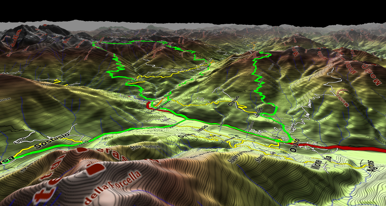
To understand the handling of the 3D-View some basic things have to be mentioned. A 3D-View is defined by the camera position (latitude/longitude/height), the viewing direction (elevation/azimut) of the camera and its zoom. You can define parameters of the environment (superelevation,fog) and picture size (width/height).
Based on this Data it is possible to assign every pixel of the picture a point on the map. To colour the 3D-View this map has to be known and is pre calculated as the texture. You might change the 'Map->settings' or change the track, now you want to update the 3D-View. This actually means updating the texture by pressing 'retexture'. If you only want to change camera position or fog or super elevation 'render' is sufficient.
When pressing '3D-View->show 3D' an default view will be rendered. It represents the view from bottom left corner of the map to the top right corner. If you see nothing, you should first try to set the 'height pos' to a reasonable value. If you enlarge the picture size you also see more. Once you see the terrain you can define a new camera position by left-click onto the picture. With right-click you can define the point where the camera should look. Of course you can type the related parameters by hand.
When you are satisfied with the picture composition you can adjust the texture. You can increase the 'Texture Megapixel' value as far as your computer allows. For a nice view you may turn off the scale in the 'Map->settings'. The fog can be defined by two values. The offset specifies a distance (in meters) where no fog at all should be considered. All terrain within this distance shows full saturation of colours. Pixels beyond this offset are desaturated exponentially with respect to its distance.